[ad_1]

Recently, I visited a friend who was working on a printout that was obviously generated by a spreadsheet application. It was a list of customer names and addresses sorted by ZIP Code, and my friend was manually counting how many customers were in each ZIP Code region. I hate to see users waste time doing something manually that could be done with software.
SEE: Google Workspace vs. Microsoft 365: A side-by-side analysis w/checklist (TechRepublic Premium)
Naturally, I had to stick my nose into the process and point out that there’s a much better way to get those numbers. In this tutorial, I’ll show you what I showed them: How to use Excel’s COUNTIF() function to return the number of times a specific value — in this case, ZIP Codes — occurs in a list. Along the way, you’ll also learn the basics of COUNTIF() so you can use this versatile function with your own work. Then, we’ll use SUBTOTAL() to count when filtering.
For this demonstration, I’m using Microsoft 365 on a Windows 10 64-bit system, but you can also use this function with earlier versions of Excel. Microsoft Excel for the web supports both of the functions we’ll be working with here.
Jump to:
COUNTIF arguments
Before we use either function, let’s look at the COUNTIF() arguments. COUNTIF() returns the number of cells that meet a specific condition that you specify. In our case, we’re counting the number of times a specific ZIP code occurs in a specified range.
COUNTIF() uses the following syntax:
COUNTIF(range,criteria)
where “range” identifies the list of values you are counting and “criteria” expresses the condition for counting.
Before we go any further, it’s important to know that COUNTIF() has one limitation. The criteria argument is limited to 255 characters when using a literal string value. It’s doubtful you’ll run into this limitation, but if you do, you can concatenate strings using the concatenation operator & to build a longer string.
Troubleshooting COUNTIF
If the COUNTIF() function returns nothing and you know the values exist, consider the following actions and tips:
- Be sure to delimit values: For example, “apples” will count the number of times the word apple appears in the referenced range; if you omit the quotation marks, it won’t work. Numeric values don’t require a delimiter, except for dates, which use the
#delimiter. - Check the values: Your referenced range may have an unnecessary space character before or after other characters. Use TRIM() to return only the values you want.
- Check if your file is open: If COUNTIF() refers to another workbook, that file must be open. Otherwise, the function returns the #VALUE! error.
- Take a closer look at your criteria text: COUNTIF() criteria values aren’t case sensitive. However, curly quotes in criteria will return an error, so if you’re pasting a value, be careful. In general, this shouldn’t be an issue.
- Don’t rely on cell formatting: COUNTIF() can’t count cells based on fill or font color values.
Now that you’re familiar with this function, let’s put it to use with a simple example.
How to use the COUNTIF function in Excel
Let’s start with a simple use of COUNTIF(). As you can see in Figure A, the function
=COUNTIF(Table1[ZIPS],10123)
returns the value of 2.
Figure A
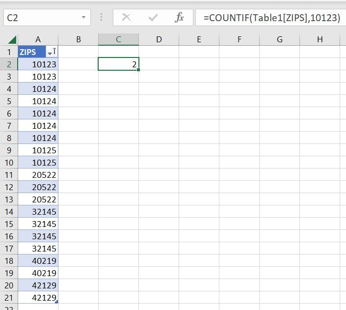
That’s because the ZIP Code value, 10123, occurs twice in the Table named Table1. If you’re not using a Table object, use the range reference as follows:
=COUNTIF(A2:A21,10123)
If you’re not familiar with structured referencing, Table1[ZIPS] might confuse you. The example data is formatted as an Excel Table object. Table1 is the Table object’s name and [ZIPS] is the column name.
Specifying a single ZIP Code is easy, but you’ll likely want to expand on this count by including all of them.
How do I count multiple items in Excel?
You can specify a literal value when using COUNTIF(), but the criteria argument supports a cell or range reference.
To demonstrate this function’s flexibility, we’ll count the number of occurrences of each ZIP Code in the sample data. Usually, ZIP Codes will accompany other address values such as name, address, city and state. We’re keeping our example simple on purpose, because those values are irrelevant when you’re counting only ZIP Code values.
SEE: Microsoft 365 Services Usage Policy (TechRepublic Premium)
If you’re using Microsoft 365, use the following expression to generate a unique list of sorted ZIP Code values (Figure B):
=SORT(UNIQUE(Table1[ZIPS]))
Figure B
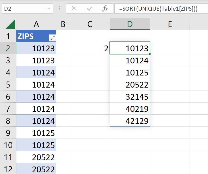
SORT() and UNIQUE() are both dynamic array functions, available only in Excel 365. In our example, there’s only one expression, which is in D2. However, the expression spills over into the cells below to fulfill the returned values as an array. If you get a spill error, there’s something blocking the array in the cells below the expression.
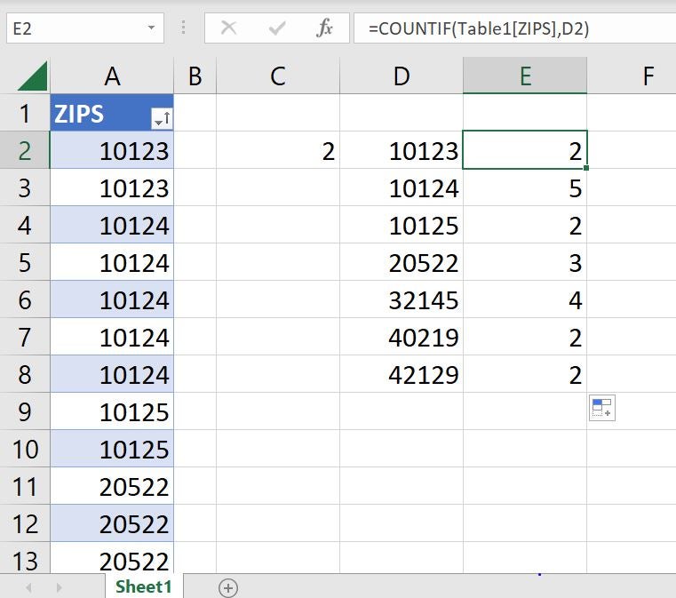
Once you have a unique list of ZIP Codes, you can use COUNTIF() to return the count of each ZIP Code value, as shown in Figure C, using
=COUNTIF(Table1[ZIPS],D2)
and copying it to the remaining cells.
Figure C
To learn more about dynamic arrays, you can read How to create a sorted unique list in an Excel spreadsheet.
How do I count multiple items in Excel pre-365?
For users who are using an earlier version of Excel than Excel 365, you’ll have to work a bit harder for the same results. If it’s important to you that the unique list of ZIP Codes is sorted, sort the source data before going any further.
To do so, you can simply click on any of the cells in column A and click the Sort Ascending button in the Sort & Filter group on the Data tab. Alternatively, you can click Sort & Filter in the Editing group on the Home tab.
To create a unique list of ZIP Codes from the values in column A, do the following:
- Click any group of cells in the dataset — in this example, we’ve selected A1:A21.
- Click the Data tab and then click Advanced in the Sort & Filter group.
- Click the Copy to Another Location option.
- Excel will display $A$1:$A$21 as the List Range. If it does not do this, you can fix it manually.
- Remove the Criteria Range if there is one.
- Click Copy To control and then click an unselected cell, such as G1.
- Check the Unique Records Only option (Figure D).
Figure D
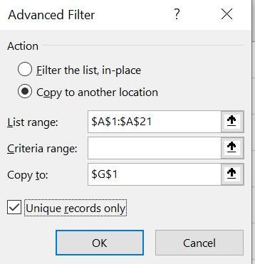
- Click OK.
This feature also copies the heading text from A1 and the formatting. There’s no way around either of these copies, but that’s okay, because neither interferes with our task.
At this point, all that’s left is the function for counting unique entries in column A based on entries in the unique list in column G. Now it’s time to enter the following function into cell H2:
=COUNTIF(Table1[ZIPS],G2)
You’ll then copy it to the remaining cells. As you can see in Figure E, this function returns the same counts as the first.
Figure E
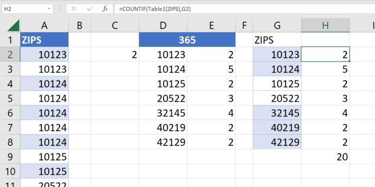
Did you notice the bold 20 in cell H9? That’s a SUM() function, which ensures the number of counted entries equals the number of original entries. Since we had 20 entries in our source data in column A, we’d expect the total number of unique entries counted to be the same.
COUNTIF() is a helpful way to count specific values in a list, but you may also run into situations where you want to count items in a filtered list. Let’s cover how to do that next.
How do I count filtered lists in Excel?
Using COUNTIF() works great in many situations, but what if you want a count based on the results of a filtered list? In this situation, the COUNTIF() function won’t work for you. The function will continue to return the correct results, but it won’t return the correct count for the filtered set. Instead, you’ll want to use the SUBTOTAL() function to count a filtered list.
Excel’s SUBTOTAL() function is rather special, as it accommodates filtering. Specifically, regardless of the mathematical calculation, this function evaluates only the values that make it to the filtered list. This function uses the following syntax:
SUBTOTAL(number,reference)
“Number” identifies the mathematical calculation and “reference” specifies the values. By default, number is 109, which is SUM(). Refer to Table A for a complete list of number values:
Table A
| Includes hidden rows | Excludes hidden rows | Function |
|---|---|---|
| 1 | 101 | AVERAGE |
| 2 | 102 | COUNT |
| 3 | 103 | COUNTA |
| 4 | 104 | MAX |
| 5 | 105 | MIN |
| 6 | 106 | PRODUCT |
| 7 | 107 | STDEV |
| 8 | 108 | STDEVP |
| 9 | 109 | SUM |
| 10 | 110 | VAR |
| 11 | 111 | VARP |
In the last section, COUNTIF() didn’t care whether the source data was a normal data range or a Table object. For this solution to work, you must work with a Table object. To convert a data range into a Table object, click anywhere inside the data range and press Ctrl + T and click OK to confirm the conversion. Doing so automatically displays a filter dropdown in the header cell.
Before we start filtering, we must add a special row to the Table as follows:
- Click anywhere inside the Table.
- Click the contextual Table Design tab.
- In the Table Style Options group, click the Total Row item (Figure F).
Figure F
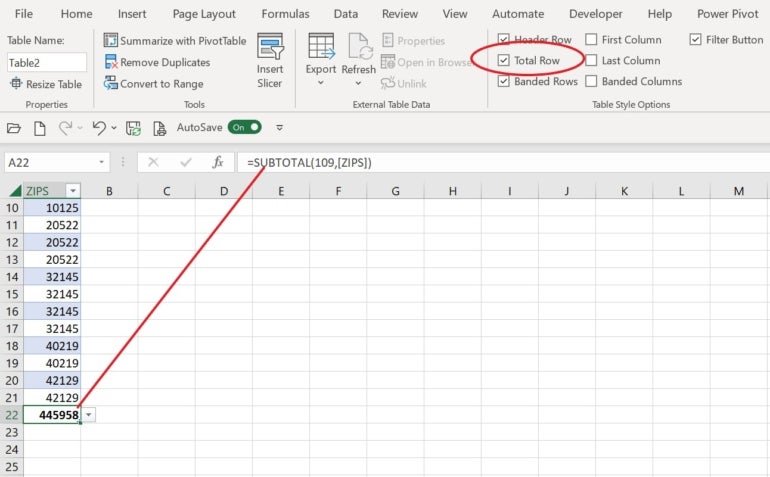
As you can see in Figure F, this row defaults to a SUBTOTAL() function that totals values by default. In this case, we don’t want a total but rather a count. To change the SUBTOTAL() function’s argument, click A22 and choose Count from the dropdown list shown in Figure G.
Figure G
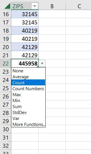
As you can see, there are many different functions you can choose. Figure H shows the count, which is 20.
Figure H
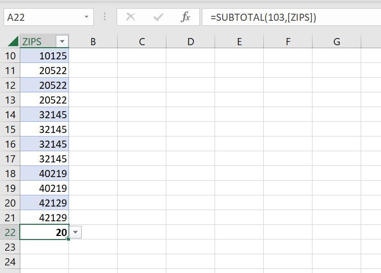
The original SUBTOTAL() function’s first argument is 109, which represents SUM(). When you change the total function to Count, SUBTOTAL() updates that argument to 103, which represents COUNT().
Start the filtering process
Once the total row is in place and displaying the count, you’re ready to begin filtering. To start, try clicking the filtering dropdown in A1 and do the following:
- Uncheck (Select All).
- Check the 10125 option (Figure I).
Figure I
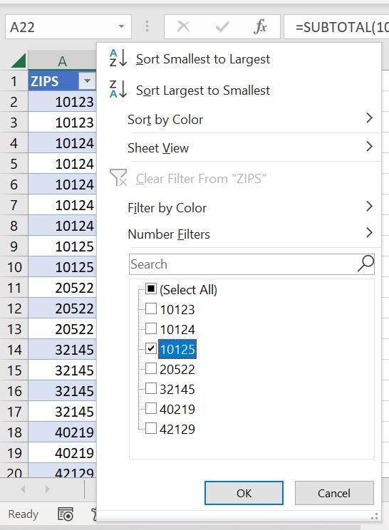
- Click OK.
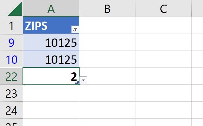
As you can see in Figure J, the filtered set includes two items, and the SUBTOTAL() function now returns two instead of 20. This function is special because, unlike other functions, SUBTOTAL() updates when you apply a filter.
Figure J
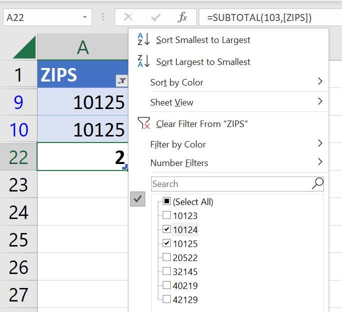
Let’s try it again, only this time, check two ZIP Codes (Figure K).
Figure K
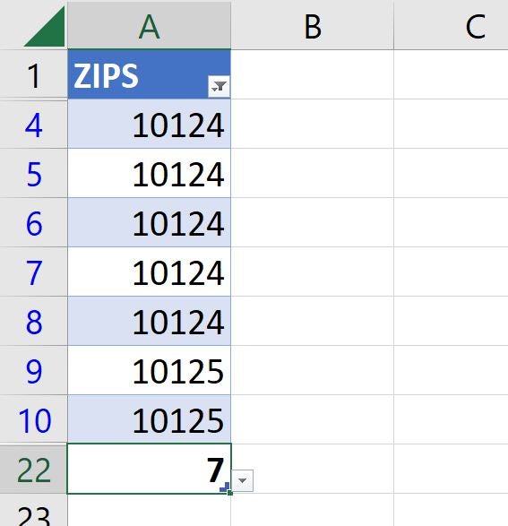
As you can see in Figure L, SUBTOTAL() returns the count of both ZIP Code values, which is 7. SUBTOTAL() is flexible enough to handle any filter you apply using the advanced filter feature.
Figure L
Additional resources
Whether you use COUNTIF() or SUBTOTAL() via a Table object’s total row, counting values is easy work. To learn more about counting, this other TechRepublic tutorial can help: How to use the UNIQUE() function to return a count of unique values in Excel.
Read next: The 8 best alternatives to Microsoft Project (Free & Paid) (TechRepublic)
[ad_2]
Source link